Tutorial 0 : getting started
This turial presents the basic usage of deepvisiontools. Each items goes step by step but you have a fully functionnal example in the section Putting everything together.
deepvisiontools is a library, overlay of pytorch, that provides high and low levels functionnalities for training deep learning detection models (bounding boxes and/or instance segmentation).
to install deepvisiontools, make sure to create a new virtual python environnment. deepvisiontools has mostly been tested under python 3.11 and 3.12.9 and therefore should work in this version range.
In your freshly created environnment run
pip install deepvisiontools
Alternatively you can clone the git repo from https://forgemia.inra.fr/ue-apc/librairies/python/deepvisiontools
Let’s get started with deepvisiontools !
Library configuration
deepvisiontools is using an overall configuration parametrization. You can setup some parameters that will control your model training, metrics computation etc.
[1]:
from deepvisiontools import Configuration

config = Configuration(device="cuda", data_type="bbox", num_classes=1)
config.model_confidence_threshold = 0.5
config.model_max_detection = 200
/home/jbernigauds/miniconda3/envs/deepvisiontools_v1/lib/python3.11/site-packages/tqdm/auto.py:21: TqdmWarning: IProgress not found. Please update jupyter and ipywidgets. See https://ipywidgets.readthedocs.io/en/stable/user_install.html
  from .autonotebook import tqdm as notebook_tqdm
As you can see, you can declare your configuration when initializing for the first time the Configuration class. Later on, if you want to modify the configuration you’ll need to change the different attributes/properties of the class (like in the second and third lines example).
The three most important parameters to play with are the ones provided in the first line : - device : can be either “cuda” or “cpu” to either run on your GPU or on your cpu - data_type : can be either “bbox” or “instance_mask”. Here we want to work with bounding boxes. Please note that additional data_types might be included in the future. Note as well that everything that works with bbox will work with instance mask (for example you can use “bbox” on your instance mask dataset) but the contrary is not true (you can always infer bounding boxes from mask but not in the other way). Using instance masks as data_type even if training a bounding box detection model can be useful, in particular for handling augmentations such as rotations for example. - num_classes : is the number of different classes of your objects.
Finally, let’s precise that all parameters in Configuration are detailed in the documentation.
Format, Dataset, Reader and Dataloader
To train a model on your dataset, you need a way to load your images and annotations and provide them to the model. In pytorch this is typically done through the implementation of your own Dataset class. Here we provide an already prepared DeepVisionDataset class. There is a default structure that is recognized for reading your data and it goes as follow :
. Dataset Name
        ├── images
            ├── name01.png
            ├── name02.png
            └── ...
        └── coco_annotations.json
where coco_annotations.json is a json file that contains your annotation as per COCO format (a dict with 3 keys : images, annotations, categories. Each key leads to a list and each element of the list is a dict with various information.). If you wish to adapt to your own dataset structures you can create your own Reader class and pass it as a DeepVisionDataset’s argument, but this require some python knowledge (a tutorial dedicated to this aspect is available).
To create your dataset :
[ ]:
from deepvisiontools import DeepVisionDataset


path_to_dataset = "path/to/dataset"
dataset = DeepVisionDataset(path_to_dataset)

for image, target, image_name in dataset:
    print(type(image), type(target), image_name)
    break
<class 'torch.Tensor'> <class 'deepvisiontools.formats.formats.BboxFormat'> Crop__20TO_IPHARD__20-07-2020__001_1_1_DSC011525__.png
You can see that the dataset will return a triplet of items for each index containing the image as a torch Tensor, the target as a deepvisiontools format and the associated image. We are going to investigate a bit later the format in deepvisiontools, but for now let’s just say that it contains all information of your annotation (here it’s a bounding box).
It’s important to note that DeepVisionDataset are by default preprocessing images (Normalizing as per ImageNet dataset). You can modify this, either implementing your own preprocessing or switching it to None when declaring your dataset or after by modifying the corresponding attribute.
DeepVisionDataset has it’s own useful methods. One of the most useful one is the possibility to randomly split the dataset :
[3]:
print("size of original dataset : ", len(dataset))
train_set, val_set, test_set = dataset.split((0.6, 0.2, 0.2))
print("size of the newly splitted datasets", len(train_set), len(val_set), len(test_set))
size of original dataset :  425
size of the newly splitted datasets 255 85 85
DeepVisionDataset can also be exported to the default structure (a folder containing an image folder and a coco_annotations.json file) by doing
[ ]:
test_set.preprocessing = None
test_set.export_dataset("path/to/export/dataset")    # Careful to not give the same name as original dataset
This function also creates visualizations by default for your exported dataset (you can choose the number of visualization by modifying the corresponding number_visu parameter in the function).
Now let’s have a look at the Format class in deepvisiontools. The key idea is that all data are handled by dedicated classes that take care of augmentation, padding, cropping, labels managements.
[5]:
img, target, _ = dataset[13]    # Load the 13 item
print("target type : ", type(target))
print("target nb of objects : ", target.nb_object)
print("target canvas_size (size of associated image) : ", target.canvas_size)
print("target data type : ", type(target.data))
print("target data value : ", target.data.value)
print("target objects class labels: ", target.labels)
print("target object scores : ", target.scores)
target type :  <class 'deepvisiontools.formats.formats.BboxFormat'>
target nb of objects :  24
target canvas_size (size of associated image) :  (768, 768)
target data type :  <class 'deepvisiontools.formats.base_data.BboxData'>
target data value :  BoundingBoxes([[  0,   0,  67,  65],
               [ 93,   0, 105,  64],
               [182,   0, 115,  75],
               [309,   0, 120,  69],
               [547,   0,  81,  46],
               [676,   0,  46,  32],
               [711, 190,  56,  77],
               [605, 213,  53,  57],
               [466, 185, 137, 114],
               [360, 187, 120, 124],
               [273, 191,  99, 121],
               [145, 200, 104, 103],
               [  0, 209,  78, 134],
               [107, 443, 113, 113],
               [202, 436, 134, 129],
               [326, 435, 120, 130],
               [453, 447, 103, 101],
               [751, 475,  16,  13],
               [703, 703,  64,  59],
               [589, 705,  77,  62],
               [449, 677, 120,  90],
               [369, 697,  80,  70],
               [135, 708, 104,  59],
               [ 54, 707,  77,  60]], device='cuda:0', format=BoundingBoxFormat.XYWH, canvas_size=(768, 768))
target objects class labels:  tensor([0, 0, 0, 0, 0, 0, 0, 0, 0, 0, 0, 0, 0, 0, 0, 0, 0, 0, 0, 0, 0, 0, 0, 0], device='cuda:0')
target object scores :  None
As you can see, the BboxFormat class has several attributes, and more generally every formats inherits from a BaseFormat class and therefore exhibits the same attributes and methods : - nb_object : is the number of object present in the format. - canvas_size : is the size of the associated image - data : this is the data saved as a particular class, child class of BaseData. To access his actual tensor value you can to format.data.value. Here you can see that the value is a
torch.Tensor and more specifically a BoundingBoxes tensor from torchvision. - labels : it’s a 1D torch.Tensor that gives the class of the associated object. - scores : it’s a 1D torch.Tensor that gives the prediction score (confidence) of the associated object. Scores is not None in case of a prediction (output of model).
A Format encapsulate many objects and usually is associated to a given image. They are used in both targets for the models and predictions of the models.
Let’s now have a look at the DeepVisionLoader class. In Pytorch, you create your dataset that will load every image - target from your data and later use a dataloader that will create batches with your dataset. In deepvisiontools we do the same but the loader is already defined so it fits the formats described above.
[6]:
from deepvisiontools import DeepVisionLoader

train_loader = DeepVisionLoader(train_set, batch_size = 4)
val_loader = DeepVisionLoader(val_set, batch_size=4)
for imgs, targs, names in train_loader:
    print(imgs.shape)
    print(type(targs))
    print(targs.formats)
    print(names)
    break
torch.Size([4, 3, 768, 768])
<class 'deepvisiontools.formats.formats.BatchedFormat'>
[<deepvisiontools.formats.formats.BboxFormat object at 0x710c0f2320d0>, <deepvisiontools.formats.formats.BboxFormat object at 0x710c0f232310>, <deepvisiontools.formats.formats.BboxFormat object at 0x710c0f232690>, <deepvisiontools.formats.formats.BboxFormat object at 0x710c0f2327d0>]
{0: 'Crop__21TE42__28-07-2021__Y02X11_DSC02087__.png', 1: 'Crop__23TE43__25-05-2023__Y02X003_DJI_202305251437150646__.png', 2: 'Crop__21TE42__03-08-2021__Y03X25_DSC03342__.png', 3: 'Crop__21TE42__28-07-2021__Y02X34_DSC02059__.png'}
As you can see, each batch of the DeepVisionLoader returns a set of stacked image (you can see that the first dim is 4 which corresponds to the batch_size we chose), a BatchedFormat that contains a format list within its formats attribute and a batch of names as a dictionnary where the key is the index in the batch.
Data augmentation
Data augmentation in deepvisiontools is handled directly in the dataset. You simply needs to provide torchvision.transforms.v2.Transform objects as a list to your dataset and everything will go smoothly. You can also include one of the additional augmentation present in deepvisiontools.
[ ]:
import torchvision.transforms.v2 as T
from deepvisiontools.data.additional_augmentations import RandomPadAndResize

augment = [T.RandomHorizontalFlip(), T.ColorJitter(brightness=0.2, contrast=0.2, saturation=0.2, hue=0.2), RandomPadAndResize((300, 300, 300, 300), (768, 768), p=0.3)]

augmented_dataset = DeepVisionDataset(path_to_dataset, preprocessing=None, augmentation=augment)
augmented_train, _, _ = augmented_dataset.split((0.1, 0.9, 0.0))
augmented_train.export_dataset("path/to/export/dataset")
Exporting dataset : 100%|██████████| 42/42 [00:44<00:00,  1.05s/it]
Grouping jsons : 100%|██████████| 78/78 [00:00<00:00, 16548.09it/s]
If you wish to change your augmentation after dataset creation you can simply change the corresponding attribute
[ ]:
augmented_train.augmentation = [ T.RandomRotation(45, expand=True),T.Resize((768, 768))]
augmented_train.export_dataset("/new/exported/dataset")
Exporting dataset : 100%|██████████| 42/42 [00:33<00:00,  1.24it/s]
Grouping jsons : 100%|██████████| 78/78 [00:00<00:00, 16951.07it/s]
Important : You can see that rotations are not super nice on boxes !! Indeed, they are now larger than the actual object. This was expected : un-oriented Bounding boxes are not invariant under the rotations, being defined by only 2 points in space. Therefore we recommend to not use rotation on bounding boxes. However rotations are perfectly fine when dealing with instance masks (check configuration).
Models, Trainer, metrics and monitoring
We can now reach the core of deepvisiontools functionnality : training and evaluating your models. Most of these aspects are handled by the Trainer class. You need however to choose the deepvisiontools model you wish to train and your favourite pytorch optimizer first.
[9]:
from deepvisiontools.models import Yolo
from torch.optim import Adam

model = Yolo("yolox")
optim = Adam(model.parameters(), lr=1e-4)   # here you tell Adam to optimize your model parameters as well as the used learning rate
Overriding model.yaml nc=80 with nc=1

                   from  n    params  module                                       arguments
  0                  -1  1      2320  ultralytics.nn.modules.conv.Conv             [3, 80, 3, 2]
  1                  -1  1    115520  ultralytics.nn.modules.conv.Conv             [80, 160, 3, 2]
  2                  -1  3    436800  ultralytics.nn.modules.block.C2f             [160, 160, 3, True]
  3                  -1  1    461440  ultralytics.nn.modules.conv.Conv             [160, 320, 3, 2]
  4                  -1  6   3281920  ultralytics.nn.modules.block.C2f             [320, 320, 6, True]
  5                  -1  1   1844480  ultralytics.nn.modules.conv.Conv             [320, 640, 3, 2]
  6                  -1  6  13117440  ultralytics.nn.modules.block.C2f             [640, 640, 6, True]
  7                  -1  1   3687680  ultralytics.nn.modules.conv.Conv             [640, 640, 3, 2]
  8                  -1  3   6969600  ultralytics.nn.modules.block.C2f             [640, 640, 3, True]
  9                  -1  1   1025920  ultralytics.nn.modules.block.SPPF            [640, 640, 5]
 10                  -1  1         0  torch.nn.modules.upsampling.Upsample         [None, 2, 'nearest']
 11             [-1, 6]  1         0  ultralytics.nn.modules.conv.Concat           [1]
 12                  -1  3   7379200  ultralytics.nn.modules.block.C2f             [1280, 640, 3]
 13                  -1  1         0  torch.nn.modules.upsampling.Upsample         [None, 2, 'nearest']
 14             [-1, 4]  1         0  ultralytics.nn.modules.conv.Concat           [1]
 15                  -1  3   1948800  ultralytics.nn.modules.block.C2f             [960, 320, 3]
 16                  -1  1    922240  ultralytics.nn.modules.conv.Conv             [320, 320, 3, 2]
 17            [-1, 12]  1         0  ultralytics.nn.modules.conv.Concat           [1]
 18                  -1  3   7174400  ultralytics.nn.modules.block.C2f             [960, 640, 3]
 19                  -1  1   3687680  ultralytics.nn.modules.conv.Conv             [640, 640, 3, 2]
 20             [-1, 9]  1         0  ultralytics.nn.modules.conv.Concat           [1]
 21                  -1  3   7379200  ultralytics.nn.modules.block.C2f             [1280, 640, 3]
 22        [15, 18, 21]  1   8718931  ultralytics.nn.modules.head.Detect           [1, [320, 640, 640]]
YOLOv8x summary: 365 layers, 68,153,571 parameters, 68,153,555 gradients, 258.1 GFLOPs

Transferred 589/595 items from pretrained weights
Be careful that some models are unusable depending of the data_type you chose in Configuration (for exemple YoloSeg cannot be used on bounding boxes). deepvisiontools did not create the models you are going to use. Please repsect the developpers of the different models and cite them in the proper way in case you want to publish results based on them. Details on every models can be find in the documentation. Specifics models will have their own tutorial as they rely on tricky
configurations that requires a bit of knowledge in models architecture.
We can now choose specific metrics to monitor our training. You can choose amoung deepvisiontools list or create your own but this require a bit of work (dedicated tutorial for that).
Once that’s done, you can instantiate your trainer :
[ ]:
from deepvisiontools import Trainer
from deepvisiontools.metrics import DetectF1score, DetectPrecision, DetectRecall

metrics = [DetectF1score(), DetectPrecision(), DetectRecall()]
trainer = Trainer(model, optim, metrics=metrics, log_dir="path/to/logdir")
The log_dir parameter is the directory name that will be created with the monitoring data will be saved. We use tensorboard to monitor the training. If you are using VScode you can install the tensorboard plugin or in your terminal with your python environment activated, where deepvisiontools is installed, go to the location of the log_dir (after starting the training) and simply run
tensorboard --logdir=log_dir
It will print you a localhost https link that you can open to monitor your training (needs to refresh to update during the epochs).
Now we have to write the training loop. To do so let’s ensure first that : - We have a training set with preprocessing and augmentation switched on - We have a valid set with preprocessing on and augmentation off
Then we can simply train our model using :
[11]:
train_set, valid_set, _ = DeepVisionDataset(path_to_dataset, augmentation=augment).split((0.5, 0.2, 0.3))
Nb_epoch = 3   # Number of epochs

valid_set.augmentation = None

train_loader = DeepVisionLoader(train_set, batch_size = 4)
valid_loader = DeepVisionLoader(valid_set, batch_size = 4)

for e in range(Nb_epoch):
    trainer.train_epoch(train_loader, e)
    trainer.valid_epoch(valid_loader, e)
Epoch 0/Train: 100%|██████████| 53/53 [00:23<00:00,  2.26it/s, loss : 2.706 loss_box : 0.207 loss_cls : 0.213 loss_dfl : 0.256 ]
Epoch 0/Valid: 100%|██████████| 22/22 [00:06<00:00,  3.62it/s, loss : 2.145 loss_box : 0.174 loss_cls : 0.136 loss_dfl : 0.244 DetectF1score : 0.927 DetectPrecision : 0.946 DetectRecall : 0.909 ]
Epoch 1/Train: 100%|██████████| 53/53 [00:22<00:00,  2.33it/s, loss : 2.044 loss_box : 0.169 loss_cls : 0.11 loss_dfl : 0.232 ]
Epoch 1/Valid: 100%|██████████| 22/22 [00:05<00:00,  3.72it/s, loss : 2.028 loss_box : 0.172 loss_cls : 0.106 loss_dfl : 0.246 DetectF1score : 0.928 DetectPrecision : 0.968 DetectRecall : 0.89 ]
Epoch 2/Train: 100%|██████████| 53/53 [00:22<00:00,  2.33it/s, loss : 1.964 loss_box : 0.164 loss_cls : 0.096 loss_dfl : 0.231 ]
Epoch 2/Valid: 100%|██████████| 22/22 [00:06<00:00,  3.66it/s, loss : 1.959 loss_box : 0.162 loss_cls : 0.104 loss_dfl : 0.24 DetectF1score : 0.935 DetectPrecision : 0.959 DetectRecall : 0.912 ]
Putting everything together and saving your model
Let’s now put all pieces together.
[ ]:
from deepvisiontools import DeepVisionDataset, DeepVisionLoader, Trainer, Configuration
from deepvisiontools.models import Yolo
from deepvisiontools.data.additional_augmentations import RandomCropAndResize, RandomPadAndResize
from deepvisiontools.metrics import DetectF1score, DetectRecall, DetectPrecision
import torchvision.transforms.v2 as T
from torch.optim import Adam
import torch
from torch.optim.lr_scheduler import ExponentialLR

config = Configuration(device="cuda", data_type="bbox", num_classes=1)  # you can give it the name that you want, the important part is that the class is instanciated at the begining

data_path = "path/to/dataset"    # path to your dataset

augment = [
           T.RandomHorizontalFlip(), # randomly flip image
           T.RandomVerticalFlip(), # randomly flip image
           T.ColorJitter(brightness=0.2, contrast=0.2, saturation=0.2, hue=0.2), # change colorimetry
           T.RandomGrayscale(p=0.05), # transform to gray scale on 5% of time
           RandomCropAndResize((650, 650), (768, 768), p=0.1), # randomly crop then resize to original img size (768, 768)
           RandomPadAndResize(150, (768, 768), p=0.1)   # Randomly pad then resize
           ]

train_set, valid_set, test_set = DeepVisionDataset(data_path, augmentation = augment).split((0.6, 0.2, 0.2))    # Create your train, valid, test sets
valid_set.augmentation = None   # switch off augmentation on valid set

train_loader = DeepVisionLoader(train_set, batch_size = 4)  # create the loaders
valid_loader = DeepVisionLoader(valid_set, batch_size = 4)

model = Yolo("yolon")   # choose a model and a specific architecture

optim = Adam(model.parameters(), lr = 1e-4) # create a weight optimizer with learning rate (lr) = 1e-4

scheduler = ExponentialLR(optim, gamma = 0.95) # Exponential decrease of lr per epoch

metrics = [DetectF1score(), DetectRecall(), DetectPrecision()]  # create a metric list to be used

trainer = Trainer(model, optim, metrics = metrics, log_dir="path/to/logdir/training_model")    # create the trainer

# ======== Training loop ========
N_epoch = 5 # number of epoch
best_loss = None    # used to save best model
for e in range(N_epoch):
    trainer.train_epoch(train_loader, e)    # train epoch e
    epoch_dict = trainer.valid_epoch(valid_loader, e)   # valid epoch e -> generate an epoch dict containing metrics and losses
    scheduler.step()    # Activate decrease of lr
    loss = epoch_dict["loss"]   # extract loss from dict
    if best_loss == None : # initialize the best loss
        best_loss = loss
    elif loss < best_loss:  # if the loss is smaller than the current best loss save the model
        torch.save(model, "/path/to/save/model/best_model.pth")
/home/jbernigauds/miniconda3/envs/deepvisiontools_v1/lib/python3.11/site-packages/tqdm/auto.py:21: TqdmWarning: IProgress not found. Please update jupyter and ipywidgets. See https://ipywidgets.readthedocs.io/en/stable/user_install.html
  from .autonotebook import tqdm as notebook_tqdm
Overriding model.yaml nc=80 with nc=1

                   from  n    params  module                                       arguments
  0                  -1  1       464  ultralytics.nn.modules.conv.Conv             [3, 16, 3, 2]
  1                  -1  1      4672  ultralytics.nn.modules.conv.Conv             [16, 32, 3, 2]
  2                  -1  1      7360  ultralytics.nn.modules.block.C2f             [32, 32, 1, True]
  3                  -1  1     18560  ultralytics.nn.modules.conv.Conv             [32, 64, 3, 2]
  4                  -1  2     49664  ultralytics.nn.modules.block.C2f             [64, 64, 2, True]
  5                  -1  1     73984  ultralytics.nn.modules.conv.Conv             [64, 128, 3, 2]
  6                  -1  2    197632  ultralytics.nn.modules.block.C2f             [128, 128, 2, True]
  7                  -1  1    295424  ultralytics.nn.modules.conv.Conv             [128, 256, 3, 2]
  8                  -1  1    460288  ultralytics.nn.modules.block.C2f             [256, 256, 1, True]
  9                  -1  1    164608  ultralytics.nn.modules.block.SPPF            [256, 256, 5]
 10                  -1  1         0  torch.nn.modules.upsampling.Upsample         [None, 2, 'nearest']
 11             [-1, 6]  1         0  ultralytics.nn.modules.conv.Concat           [1]
 12                  -1  1    148224  ultralytics.nn.modules.block.C2f             [384, 128, 1]
 13                  -1  1         0  torch.nn.modules.upsampling.Upsample         [None, 2, 'nearest']
 14             [-1, 4]  1         0  ultralytics.nn.modules.conv.Concat           [1]
 15                  -1  1     37248  ultralytics.nn.modules.block.C2f             [192, 64, 1]
 16                  -1  1     36992  ultralytics.nn.modules.conv.Conv             [64, 64, 3, 2]
 17            [-1, 12]  1         0  ultralytics.nn.modules.conv.Concat           [1]
 18                  -1  1    123648  ultralytics.nn.modules.block.C2f             [192, 128, 1]
 19                  -1  1    147712  ultralytics.nn.modules.conv.Conv             [128, 128, 3, 2]
 20             [-1, 9]  1         0  ultralytics.nn.modules.conv.Concat           [1]
 21                  -1  1    493056  ultralytics.nn.modules.block.C2f             [384, 256, 1]
 22        [15, 18, 21]  1    751507  ultralytics.nn.modules.head.Detect           [1, [64, 128, 256]]
YOLOv8n summary: 225 layers, 3,011,043 parameters, 3,011,027 gradients, 8.2 GFLOPs

Downloading https://github.com/ultralytics/assets/releases/download/v8.3.0/yolon.pt to 'yolon.pt'...
100%|██████████| 6.25M/6.25M [00:00<00:00, 11.0MB/s]
Transferred 319/355 items from pretrained weights
Epoch 0/Train: 100%|██████████| 64/64 [00:13<00:00,  4.86it/s, loss : 3.699 loss_box : 0.287 loss_cls : 0.353 loss_dfl : 0.287 ]
Epoch 0/Valid: 100%|██████████| 22/22 [00:03<00:00,  7.05it/s, loss : 3.805 loss_box : 0.244 loss_cls : 0.494 loss_dfl : 0.245 DetectF1score : 0.098 DetectRecall : 0.052 DetectPrecision : 1.0 ]
Epoch 1/Train: 100%|██████████| 64/64 [00:11<00:00,  5.39it/s, loss : 2.715 loss_box : 0.227 loss_cls : 0.21 loss_dfl : 0.245 ]
Epoch 1/Valid: 100%|██████████| 22/22 [00:03<00:00,  5.56it/s, loss : 2.76 loss_box : 0.233 loss_cls : 0.235 loss_dfl : 0.245 DetectF1score : 0.774 DetectRecall : 0.635 DetectPrecision : 0.991 ]
Epoch 2/Train: 100%|██████████| 64/64 [00:12<00:00,  5.23it/s, loss : 2.547 loss_box : 0.215 loss_cls : 0.186 loss_dfl : 0.239 ]
Epoch 2/Valid: 100%|██████████| 22/22 [00:04<00:00,  5.21it/s, loss : 2.553 loss_box : 0.231 loss_cls : 0.184 loss_dfl : 0.244 DetectF1score : 0.883 DetectRecall : 0.801 DetectPrecision : 0.984 ]
Epoch 3/Train: 100%|██████████| 64/64 [00:11<00:00,  5.37it/s, loss : 2.459 loss_box : 0.209 loss_cls : 0.172 loss_dfl : 0.237 ]
Epoch 3/Valid: 100%|██████████| 22/22 [00:04<00:00,  5.32it/s, loss : 2.449 loss_box : 0.223 loss_cls : 0.17 loss_dfl : 0.24 DetectF1score : 0.892 DetectRecall : 0.818 DetectPrecision : 0.981 ]
Epoch 4/Train: 100%|██████████| 64/64 [00:11<00:00,  5.41it/s, loss : 2.403 loss_box : 0.207 loss_cls : 0.163 loss_dfl : 0.234 ]
Epoch 4/Valid: 100%|██████████| 22/22 [00:04<00:00,  5.28it/s, loss : 2.347 loss_box : 0.21 loss_cls : 0.159 loss_dfl : 0.237 DetectF1score : 0.904 DetectRecall : 0.844 DetectPrecision : 0.974 ]
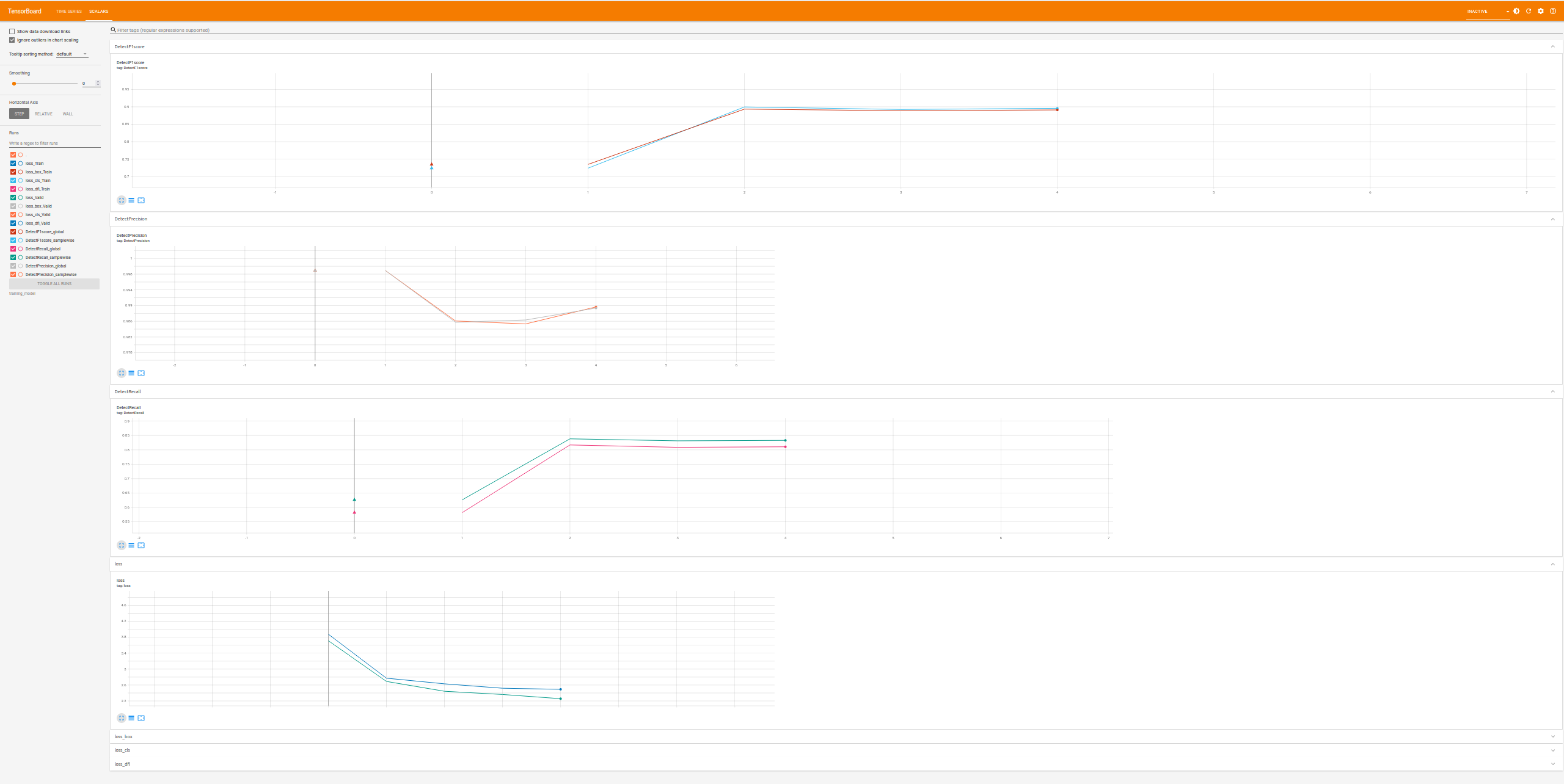
Don’t forget that you can monitor your training via tensorboard (the following is a saved image, numbers might not match …)
Inference
We can now use our model to do some predictions using deepvisiontools. To do so we are going to use the Predictor class. Note that the Predictor includes a preprocessing by default, so you need to setup the same as your training set. In our little example we are going to use the test_set from the previous piece of code and switching off the preprocessing (by default in deepvisiontools predictor and dataset have the same).
[ ]:
from deepvisiontools import Predictor

test_set.preprocessing = None   # switching off preprocessing of dataset we are going to use the predictor one
test_set.augmentation = None
image, target, _ = test_set[15] # load image and target


model = torch.load("path/to/model/best_model.pth")   # loading model
predictor = Predictor(model)    # creating the predictor with no preprocessing (image already preprocessed)

result = predictor.predict(image)   # result is a format object (as discussed previously in the first section)

print("number of predicted objects : ", result.nb_object) # number of predicted objects

# let's create a visualization !

_ = predictor.predict(image, visu_path="/path/to/visu/visu.png")
number of predicted objects : 16
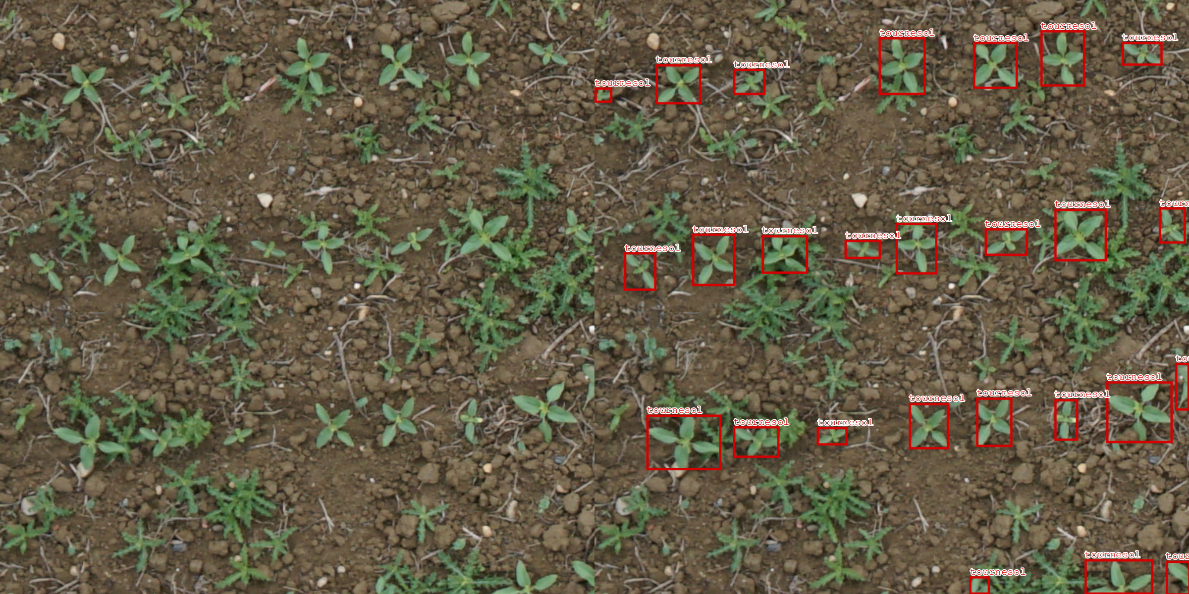
Here you got the visualization :
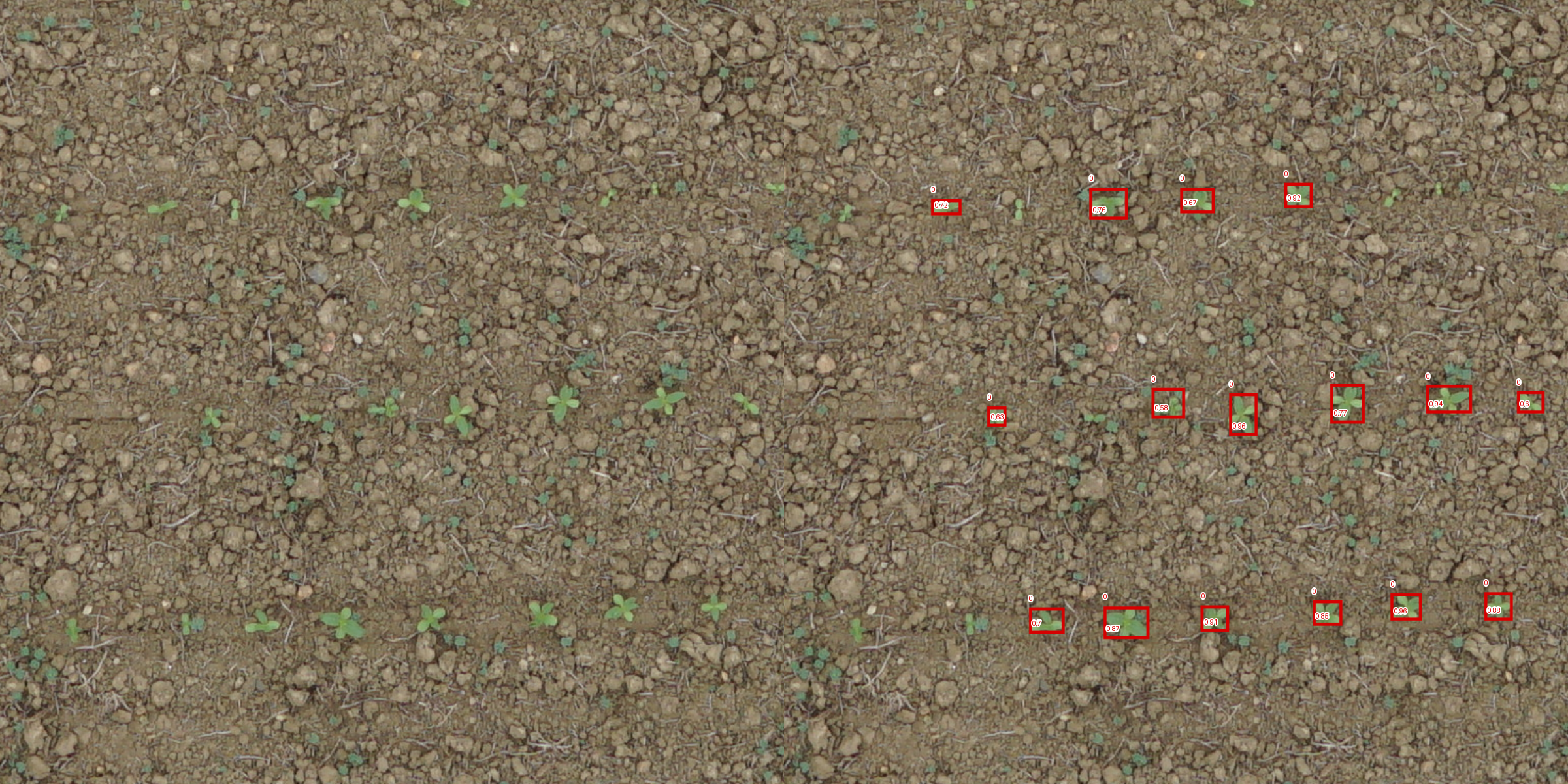
As you can see the model still makes mistakes. Of course you can now use larger models, more data, better augmentation and play with others hyper-parameters ! Have fun !